Election Sentiment Analysis

Python / Scikit-learn / NLTK / Snscrape

NB: project done in Fall 2022, X (renamed from Twitter) has overhauled their API and this project, particularly the ETL phase, would have been done differently today.

ETL & Preprocessing Pipeline

The pipeline forecasts 2016 election results using a full Extract-Transform-Load (ETL) process. We used Snscrape to harvest a large corpus of political tweets associated with the primary candidates (Clinton, Trump, Sanders, Bush), bypassing standard API limits.

Raw text required cleaning to be viable. We implemented a preprocessing chain using Regex and NLTK to normalize the dataset. This involved stripping URLs, removing user tags, normalizing repeated characters (e.g., "cooooooool" → "cool"), and filtering out standard English stopwords to reduce feature noise.

def preprocess(input_df):
    # Normalize case
    out = input_df.apply(lambda x: x.lower())
    # Remove Regex patterns (URLs, Mentions)
    out = out.apply(lambda x: clean_URLs(x))
    out = out.apply(lambda x: clean_tags(x))
    # Normalize repetition (e.g. "Runnnnn" -> "Run")
    out = out.apply(lambda x: clean_repetition(x))
    # Remove NLTK stopwords
    out = out.apply(lambda x: clean_stopwords(x))
    return out

Fig 1. The preprocessing pipeline. This function transforms raw, noisy social media text into a clean token stream ready for vectorization. We automated the extraction via Python's system interface, executing CLI queries bounded by the election cycle (2016-01-01 to 2016-11-08), ensuring that we didn't contaminate our data. The scraper targeted official candidate handles (like @realDonaldTrump) and streamed payload data directly into JSONL files to preserve metadata structure for downstream processing (e.g., if we wanted to plot sentiment for each candidate by date, etc).

Naive Bayes Classification

We utilized the Sentiment140 dataset to train our classifier. The text data was vectorized using a Binary Count Vectorizer, effectively creating a Bag-of-Words model that ignores frequency and position but tracks presence. We selected a Multinomial Naive Bayes classifier for the method of inderence. Despite the "naive" assumption of feature independence, this probabilistic model empirically excels at high-dimensional text classification.

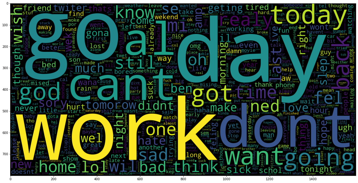
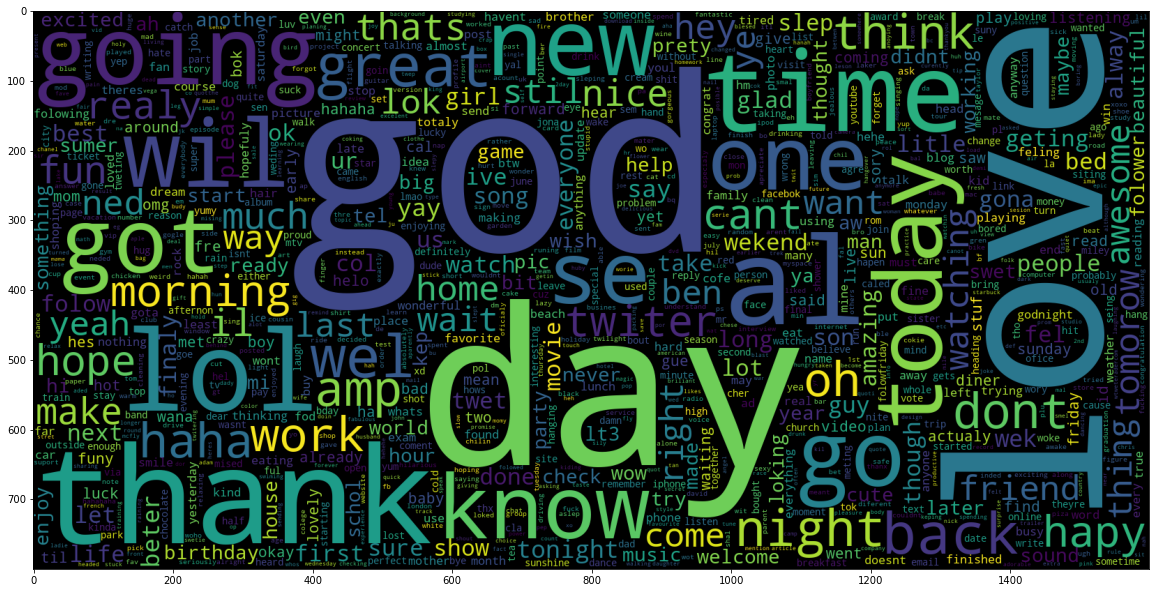
Visualizing the training data reveals distinct lexical patterns between classes. The word clouds below illustrate the most frequent tokens associated with negative and positive sentiment in the Sentiment140 dataset, serving as the basis for the model's probability distribution.

Negative Sentiment Wordcloud — Fig 2. Wordcloud generated from the negative training subset. Prominent tokens include "work,", "cant,", "dont," and "going," which the model learns to associate with negative sentiment probabilities.

Positive Sentiment Wordcloud — Fig 3. Wordcloud generated from the positive training subset. Tokens such as "love," "God," "thank," and "nice" dominate the feature space for this class.

We trained the model on a standard 80/20 train-test split, achieving an accuracy score of 77.7% on the validation set. We did not do hyperparameter tuning.

# Pipeline Definition
nb_model = make_pipeline(
    CountVectorizer(binary=True),
    MultinomialNB()
)

# Training
nb_model.fit(train_text, train_target)
model_score = nb_model.score(test_text, test_target)
print(f"Validation Accuracy: {model_score}") 
# Output: 0.77705625

Fig 4. Model instantiation using a Scikit-learn pipeline. The model learns the probability distribution of tokens associated with positive (1) or negative (0) sentiment.

Results & Thresholding

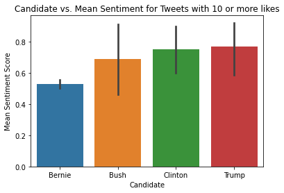
To improve signal quality, we applied an activity threshold, filtering for tweets with >10 likes. The hypothesis that high-engagement content better reflects voter intent than low-quality spam was validated by the data shift, ergo the "Threshed" metric significantly increased the mean sentiment separation between candidates.

Quantitatively, the model successfully predicted the outcomes of both the Primaries and the General Election. In the GOP primary, Trump (0.769) led Bush (0.687). In the Democratic primary, Clinton (0.750) led Sanders (0.526). Most notably for the General Election, despite close polling data at the time, the model's engagement-weighted sentiment favored Trump (0.769) over Clinton (0.750), aligning with the final Electoral College result.

Bar plot showing predicted election candidate sentiment — Fig 5. Sentiment analysis results comparing aggregate scores for candidates. The chart demonstrates that while raw sentiment scores (blue) were inconclusive, the "Threshed" data (orange) correlated accurately with the General Election outcome.